Tamm Plasmon at a Metal-DBR Interface
This case targets the Tamm-plasmon mode at a metal-dielectric Bragg reflector interface. Unlike the omnidirectional-reflector example, the objective here is not broadband high reflectance. The relevant signature is a narrow resonance dip embedded in an otherwise high-reflectance spectral region.
The geometry is still a one-dimensional stratified stack, so TMM remains the correct solver class. What changes is the sensitivity to boundary phase. In practical terms, the question is no longer "does the multilayer interfere," but "does the interface support the specific resonant feature reported in the paper."
Research Context
A Tamm plasmon is a localized optical state supported at the boundary between a metal and a periodic dielectric reflector. The DBR supplies a stop-band background, while the metal boundary supplies the additional phase condition required for a localized interface mode.
This is a natural TMM problem because the structure is still purely layered. The two observables that matter are the narrow resonance in Reflection and the depth-resolved field profile in Depth Distribution. Both are already available in Dreapex TMM without introducing any lateral patterning or grating coupling.
Paper Information and Comparison Target
- Paper: Tamm plasmon-polaritons: Possible electromagnetic states at the interface of a metal and a dielectric Bragg mirror
- Authors: M. Kaliteevski, I. Iorsh, S. Brand, R. Abram, J. Chamberlain, A. Kavokin, I. Shelykh
- Journal: Physical Review B 76, 165415 (2007)
- DOI: 10.1103/PhysRevB.76.165415
- Comparison target:
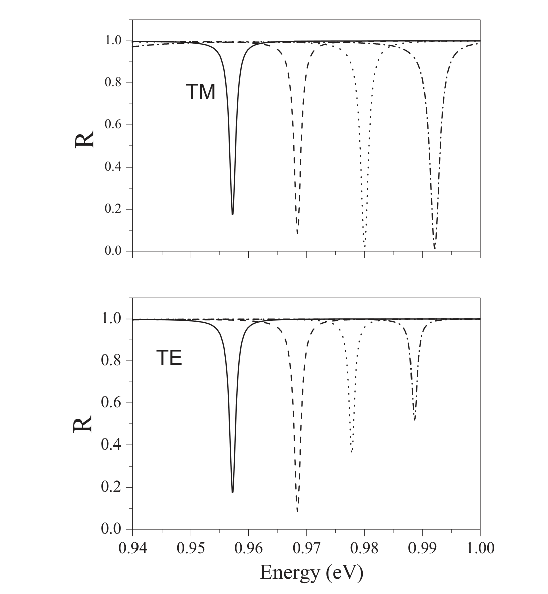
Figure 3in the paper
Figure 3 is plotted against photon energy. Dreapex TMM uses wavelength. This case therefore maps the paper's 0.94-1.00 eV window to 1240-1320 nm through
lambda (nm) ~= 1240 / E (eV).
Mapping the Paper to a Dreapex TMM Model
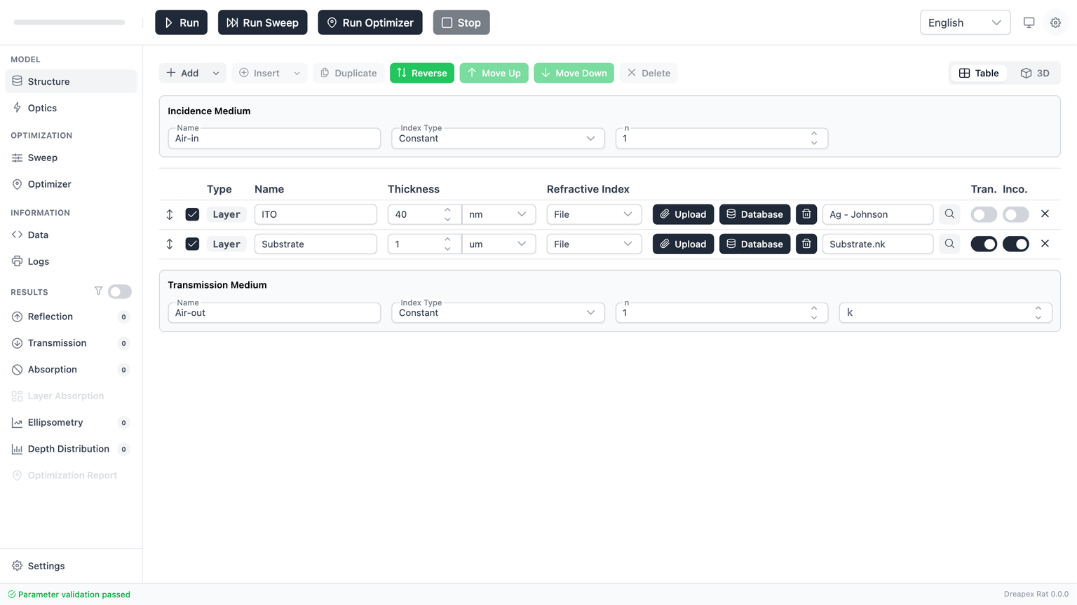
This reconstruction is performed through the live app, not by writing internal state. The structure, run sequence, and screenshots are all produced by Playwright operating the actual front end, with the Footer checked before each run to confirm that no blocking validation errors remain.
| Item | Implementation used here | Notes |
|---|---|---|
| Incidence side | Default Air incidence medium | Keeps the current UI's incident-angle control aligned with an external-angle interpretation; this is an explicit approximation relative to the paper's ideal boundary treatment |
| DBR | LayerGroup: GaAs (83.8 nm) / AlAs (103.3 nm) x 14 | First-pass reconstruction of the 14-period quarter-wave GaAs/AlAs Bragg reflector |
| Metal side | Transmission Medium = Au-backing | Approximates the paper's semi-infinite gold layer with a semi-infinite absorbing backing |
| Refractive-index sources | main/GaAs/nk/Skauli.yml, main/AlAs/nk/Fern.yml, main/Au/nk/Johnson.yml | All material data come from the built-in refractive-index database |
| Material assignment path | Standard front-end File Upload using .nk files exported from the database entries | The current LayerGroup workflow is most stable when repeated sublayers use file-backed optical data |
| Wavelength window | 1240-1320 nm, step 1 nm | Direct wavelength-space mapping of the paper's Figure 3 window |
That distinction matters: this is not an offline curve injected into the result page. The run goes through the real Structure -> Optics -> Run -> Results flow, and the screenshots preserve the app's own model configuration and validation state.
Modeling Workflow in the App
The build sequence is:
- Create a
Layer GroupinStructure. - Define the repeated unit as
GaAs / AlAs, with14periods. - Set the metal side to
Au-backing, using gold optical data sourced from the built-in database. - Check the
Footerand confirm that the status readsParameter validation passed. - In
Optics, set the wavelength window to1240-1320 nmso the scan matches the paper'sFigure 3axis.


Reproduction Target and Acceptance Criteria
For Figure 3, the evaluation criteria are:
- A clear narrow reflectance dip must appear inside the
1240-1320 nmwindow. - With increasing incident angle, the dip should shift toward shorter wavelength rather than collapse into a flat high-reflectance plateau.
- At the resonant wavelength, the depth-resolved field should preferentially strengthen near the metal-DBR boundary instead of behaving like a generic standing wave distributed through the entire stack.
In a first-pass reconstruction, satisfying the first condition places the model in the correct spectral neighborhood. Failing the second or third condition means the paper's full Tamm-plasmon branch has not yet been reproduced and should not be claimed as such.
Simulation Results vs. Paper Figure 3
Each paper panel is shown immediately next to the matching Dreapex TMM result page. This first pass tracks the TM branch only; the paper's TE panel is reproduced below with a note.
TM branch
The paper's TM panel shows a normal-incidence dip near 0.957 eV and three shifted branches at 30°, 45°, 60°. The Dreapex TMM run finds a normal-incidence minimum near 1286 nm (~0.964 eV, minimum reflectance ~0.18), placing the result in the same spectral neighborhood as the paper's normal branch.
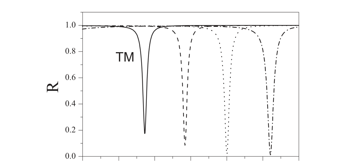

At 60°, the model returns an almost flat near-unity reflectance across the same window. The high-angle resonance branch visible in the paper does not reappear here, so the current pass is a normal-incidence resonance reconstruction rather than a full angle-dispersion reproduction.

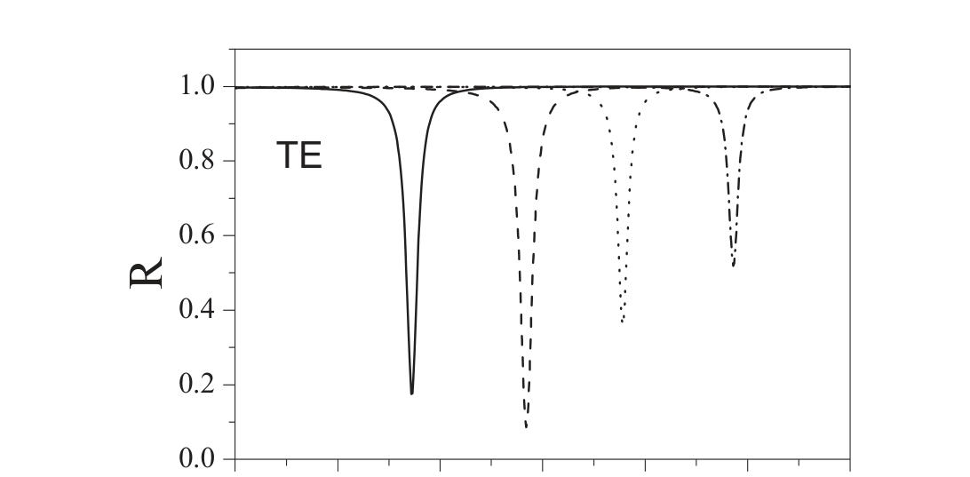
TE branch (paper only, not reproduced)
The paper also shows a TE panel with the same four angles. In this first pass the TE sweep behaves like the oblique TM case within the 1240-1320 nm window, so it is presented for reference but not claimed as a matched result.
Depth-Resolved Field Check
At normal incidence and 1286 nm, the Electric Field page shows a strong depth-selective response, but the dominant peaks are still distributed through the stack rather than pinned tightly to the first metal-DBR boundary. That is an important distinction.
It means:
- the model is exciting a strong resonance in the correct spectral neighborhood
- the resonance is not yet a clean reproduction of the ideal interface-localized Tamm-plasmon field pattern
- further tightening of the termination condition is still required before claiming full modal agreement

Deviation Analysis
The current mismatch is mainly driven by the following factors:
- the paper discusses an idealized metal-DBR boundary condition, while this case uses dispersive database materials through the real front-end solver path
- the incidence side is kept as default
Airso the UI angle control retains a direct external-angle meaning; that is not strictly identical to the boundary treatment in the analytical derivation - the 14-period
LayerGroupreproduces the base periodic stack, but the exact metal-side termination has not yet been tuned beyond the first canonical configuration - the metal side uses
Johnsongold, and different gold datasets can shift the interface phase substantially - the current wavelength step is
1 nm, which is sufficient to locate the resonance region but not to characterize a meV-scale linewidth precisely
The correct technical conclusion for this version is therefore: the live front-end workflow reproduces the normal-incidence resonance in the target spectral neighborhood, but it does not yet fully recover the angular branches or the ideal interface-localized field pattern reported in Figure 3.
Further Experiments
- Keep the same database materials and scan the metal-side termination order to test whether the oblique branches return to the
1240-1320 nmwindow. - Hold the
Figure 3window fixed and repeat the case with a different built-in gold dataset such asRakic-BB. - Refine the wavelength step below
1 nmonce the branch position is stabilized, then revisit resonance depth and linewidth. - Build a separate
30 nmfinite-gold-film version and compare it toFigure 1/Figure 4, where the finite-thickness metal configuration is closer to the paper's illustrated field profiles.
Omnidirectional Reflector
Reproduce the PS-Te nine-layer omnidirectional reflector from Fink et al. (Science, 1998) in Dreapex TMM and compare it directly against Figure 4.
Ultrathin Absorbing Interference Coatings
Reproduce the calculated reflectivity of thick Au coated with thin Ge films (5/10/15/20/25 nm) from Kats et al. (Nature Materials, 2013), Figure 2c, in Dreapex TMM.