Emitter Setup
This guide explains how to mark an emissive layer in Structure and set an Emitter spectrum, position, orientation, and efficiency. Afterward, you can create a usable light source for an emission simulation.
Marking an emissive layer
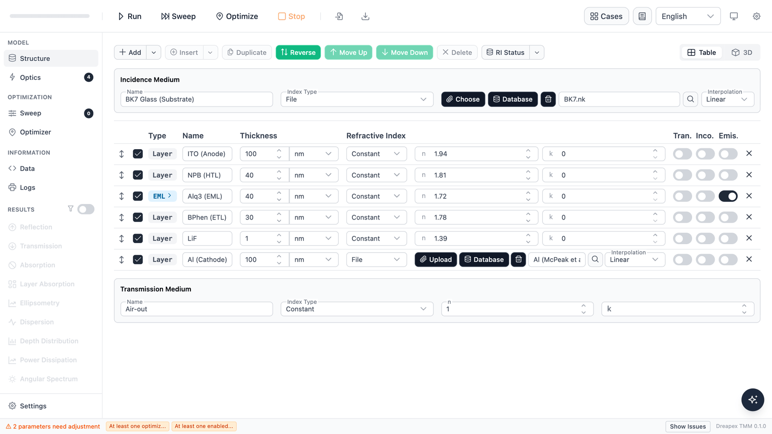
In the Structure page layer table, every Layer row has an Emis. column (header Emis.). Click the toggle switch in that column to mark the layer as an emissive layer (EML).
Toggle-on behavior
- If the layer's emitter list is empty, the system automatically seeds one default emitter (named
Emitter 1) and expands the emitter editor for that layer. - The emitter editor appears as an expansion row beneath the layer; click the EML pill in the layer type column to collapse or expand it.
Toggle-off behavior (non-destructive)
- Turning off the Emis. switch does not delete existing emitter data; the editor collapses but data is preserved.
- Re-enabling the switch restores the full emitter list.
Multi-EML support
Multiple layers can be marked as EML simultaneously. Each layer holds its own independent emitter list.
Layer Group-nested layers
Layers inside a Layer Group also support the Emis. toggle. The Optics page inspects both top-level and group-nested layers to determine whether any emissive layer (EML) is active.
Emitter editor
The emitter editor displays all emitter cards for the selected layer. Each card header provides an enable/disable toggle, move up, move down, duplicate, and delete controls; the card body is a 4-column grid containing all fields below.
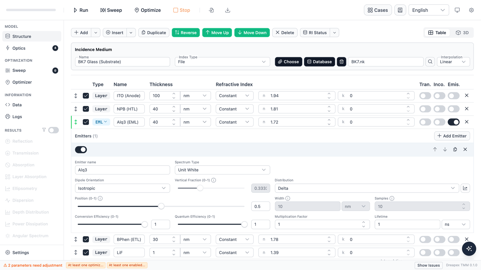
| Field | Control / Range / Unit | Meaning (1 line) |
|---|---|---|
| Emitter name | Text input; default Emitter {index} | Display label only; no physical effect |
| Spectrum Type | Dropdown: Unit White / File; default Unit White | Unit White = flat unit spectrum; File = an uploaded or generated wavelength-dependent spectrum |
| Spectrum Unit | Dropdown: Probability / Power; default Probability | Declares whether the vertical axis represents photon count or radiant power per unit wavelength |
| Spectrum File | Upload / Generate / clear / preview; shown only when Spectrum Type = File; uploads accept .txt / .pl, ≤ 2 MB, with two columns: wavelength and intensity | Upload a measured or theoretical spectrum, or generate a normalized Gaussian spectrum from peak and FWHM values |
| Dipole Orientation | Dropdown: Isotropic / Parallel / Perpendicular / Custom; default Isotropic | Orientation controls TE/TM coupling ratio and far-field angular distribution; see Dipole Model and Applicability |
| Vertical Fraction (0-1) | Slider + number input; range 0–1, step 0.01; enabled only when orientation = Custom; default ≈ 0.333 | Fraction of perpendicular (vertical) dipoles: 0 = all parallel, 1 = all perpendicular, 1/3 = isotropic |
| Distribution | Dropdown: Delta / Exponential / Gaussian / File; default Delta | Spatial profile of the emitter across the layer thickness; see Dipole distribution below |
| Position (0-1) | Slider + number input; range 0–1, step 0.01; default 0.5; hidden when Distribution = File | Relative position inside the layer: 0 = near top surface (incidence side), 1 = near bottom surface (transmission side) |
| Width | Number input + unit select (nm / um / mm); > 0; default 10 nm; disabled when Distribution = Delta | Gaussian standard deviation or exponential decay length; profile is sampled inside the layer and renormalized |
| Samples | Integer input; range 1–100; default 10; disabled when Distribution = Delta | Number of point dipoles used to approximate the distribution; Delta always uses a single point |
| Distribution File | File upload (.txt / .csv, ≤ 2 MB, 2 columns: position density); shown only when Distribution = File | Arbitrary custom emission zone profile |
| Conversion Efficiency (0-1) | Slider + number input; range 0–1, step 0.01; default 1 | Product of charge balance factor and spin-statistics factor; quantifies the probability that an injected charge pair produces an exciton. See The Light-Extraction Problem |
| Quantum Efficiency (0-1) | Slider + number input; range 0–1, step 0.01; default 1 | Intrinsic radiative quantum efficiency q₀, modified by the Purcell effect to yield the effective quantum efficiency. See Purcell Effect |
| Multiplication Factor | Number input; ≥ 0, step 0.1; default 1 | Linear scaling applied to this emitter's intensity; used to set relative weights among multiple emitters |
| Lifetime | Number input + unit select (ns / us / ms); > 0, step 0.1; default 1 ns | Intrinsic total-decay lifetime; modified by the Purcell factor to yield the effective lifetime. See Purcell Effect |
Gaussian Spectrum Generation
When only the peak wavelength, full width at half maximum (FWHM), and an approximate lineshape are available, you can synthesize a normalized Gaussian spectrum in the emitter editor without preparing a two-column spectrum file. One component provides an idealized narrowband or broadband starting point; several components can approximate shoulders, broad envelopes, and multipeak emission.
Set Spectrum Type to File, then click Generate in the Spectrum File row. The generator keeps the Gaussian components, wavelength range, and live preview in one dialog:
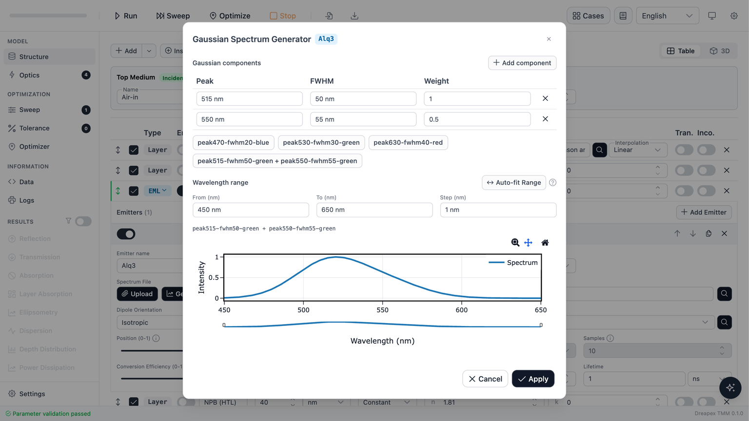
- Select a parameter preset as a starting point, or edit the components directly.
Peak,FWHM, andWeightmust each be greater than 0, and at least one component must remain. - Use
Add componentto add peaks.Weightis the relative amplitude before combination and normalization; the global maximum of the final spectrum is normalized to 1. - Set
From,To, andStep. ClickingAuto-fit Rangeonce reads the wavelength settings of all enabled detectors and fills their combined range. If no usable range exists, Dreapex TMM estimates a range that covers the tails of the current Gaussian components. - Check the live preview and click
Apply. The generated data is written to the current emitter; afterward, use the preview button at the right of the spectrum row to inspect it, add a description, or export the data.
Auto-fit Range updates the values only when clicked. Editing a component afterward does not recalculate the range, and manual range edits remain in place for the current application.
Upload for PL / EL data with vibrational fine structure, strong asymmetry, or required provenance. Clicking Apply replaces the current spectrum, and the generator does not retain the individual Gaussian components for later re-editing.Choose the spectrum unit
Probability denotes a photon-number spectrum and is appropriate for most photon-counted PL / EL measurements. Power denotes a radiant-power spectrum and should be used only for spectra calibrated as power. The two descriptions are related by the photon energy:
Here, is the energy of one photon at wavelength , is the Planck constant, and is the speed of light in vacuum. is the photon-number spectral density, while is the radiant-power spectral density. Because shorter-wavelength photons carry more energy, the same vertical-axis values declared as Probability and Power represent different physical spectra.
| Goal | Recommended setting |
|---|---|
Measured PL / EL spectrum or a typical .pl file | Probability |
| Spectrum calibrated in W/nm or another power unit | Power |
| Remove a specific PL lineshape when comparing Mode over a wavelength range | Unit White + Probability |
Unit White means constant only in the selected unit. Unit White + Probability is flat in photon number; Unit White + Power is flat in radiant power and gives progressively greater photon-number weight to longer wavelengths.
Dipole distribution
The Distribution field sets the spatial profile of emitting dipoles across the layer thickness.
| Type | Description | Width / Samples |
|---|---|---|
| Delta | Single point dipole concentrated at Position | Width and Samples are disabled (fixed single point) |
| Exponential | Peak at Position, exponential decay; Width = decay length | Both Width and Samples are configurable |
| Gaussian | Centered at Position, Width = standard deviation | Both Width and Samples are configurable |
| File | Arbitrary profile loaded from file; Position field is hidden | Width and Samples are disabled |
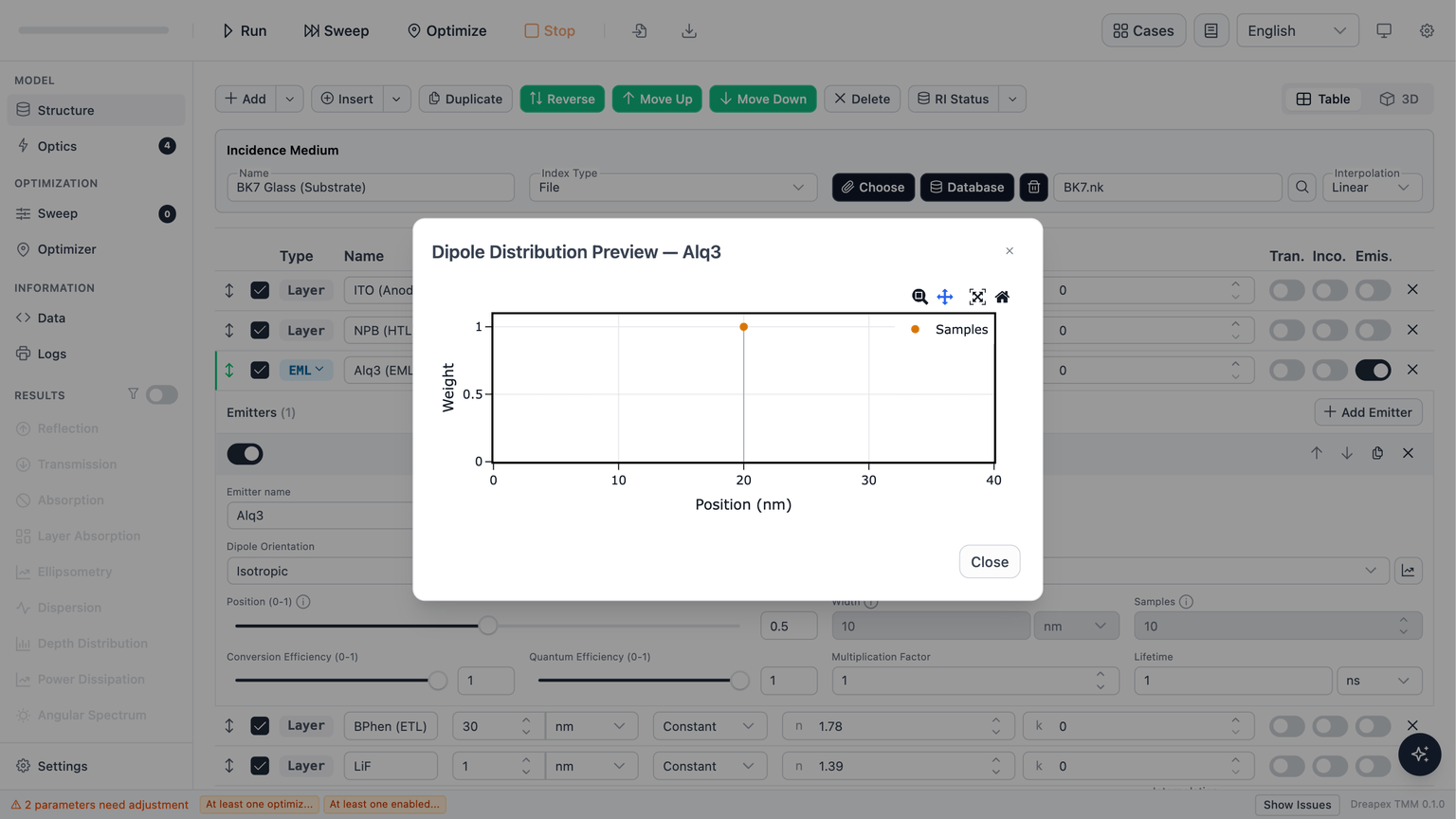
Click the preview button next to the Distribution dropdown to open a dialog showing the sampled distribution curve under the current parameters.
The distribution is sampled inside the layer and renormalized so the total integral equals 1; absolute amplitude is governed by Multiplication Factor and Conversion Efficiency independently of the profile shape.
Conversion Efficiency is the probability that recombining charges form emitting excitons. For one emitter, it scales Intensity and Power Dissipation linearly but does not change the relative Mode composition. With several emitters, different conversion efficiencies also change their relative weights in the combined Mode, spectrum, and color.
Validation
File emitter spectrum must cover the wavelength ranges of all enabled emission detectors. For a generated spectrum, click Auto-fit Range first. For an uploaded spectrum, make sure its first and last wavelengths cover the current sampling ranges of Power Dissipation, Intensity, and Mode.Next
After configuring emissive layers and their emitters, go to Emission Detectors to select which emission detectors to run (Power Dissipation, Intensity, Mode) and configure their wavelength ranges.