Principles

Power Dissipation and Optical Modes

In-plane wavevector, dissipated-power spectra, and the partition of outcoupling and loss channels

A peak in an emission power curve identifies useful outcoupling, waveguiding, or metal near-field loss only after it is placed in the correct wavevector interval. Beyond total internal reflection, the propagation angle ceases to be real, but the in-plane wavevector continues to describe the state without interruption.

The power dissipation spectrum gives the distribution of dipole energy over in-plane wavevector. Optical modes integrate that distribution across physical boundaries into outcoupling and loss fractions. They are the distribution map and the summary table of the same energy budget.

Energy Channels in a Planar Device

Electromagnetic energy from an emitting dipole can propagate upward or downward, remain trapped in the stack, be absorbed, or couple into a metal near field.

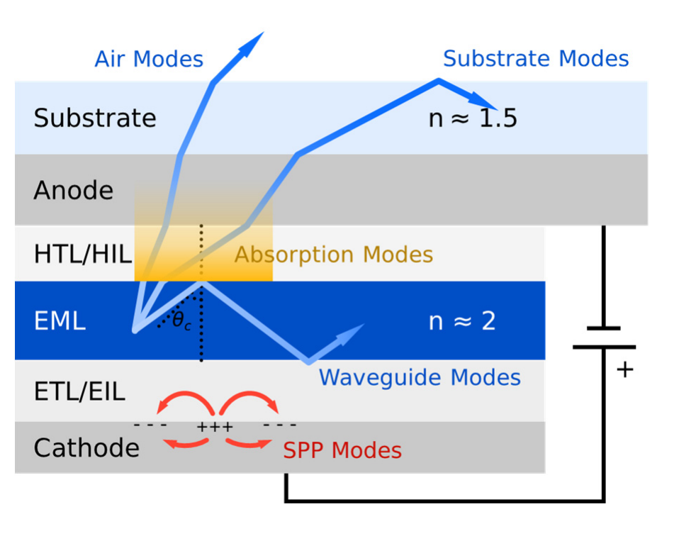
Air, substrate, absorption, waveguide, and surface-plasmon channels in a bottom-emitting device — Figure 1 | Major optical channels in a planar emitter. Every path begins at the same internal dipole source but ends in a different external medium or loss mechanism.

A ray diagram provides intuition, but guided-mode peaks, SPP peaks, and overlapping absorption must be treated in wavevector space. Translational symmetry along a planar interface conserves the wavevector component parallel to that interface throughout the stack.

Three Forms of In-Plane Wavevector

For an isotropic layer,

k_{\parallel}=n_i k_0\sin\theta_i =\frac{2\pi}{\lambda}n_{\mathrm{eff}},

and normalization to the emissive-layer index gives

n_{\mathrm{eff}}=n_i\sin\theta_i, \qquad u=\frac{k_{\parallel}}{n_e k_0} =\frac{n_{\mathrm{eff}}}{n_e}.

Here, $k_{\parallel}$ is the in-plane wavevector, $k_0=2\pi/\lambda$ is the vacuum wavenumber, $\lambda$ is vacuum wavelength, $n_i$ and $\theta_i$ are the refractive index and propagation angle in layer $i$ , $n_e$ is the emissive-layer index, $n_{\mathrm{eff}}$ is the effective index, and $u$ is the normalized in-plane wavevector. The three quantities are different scales for the same horizontal axis.

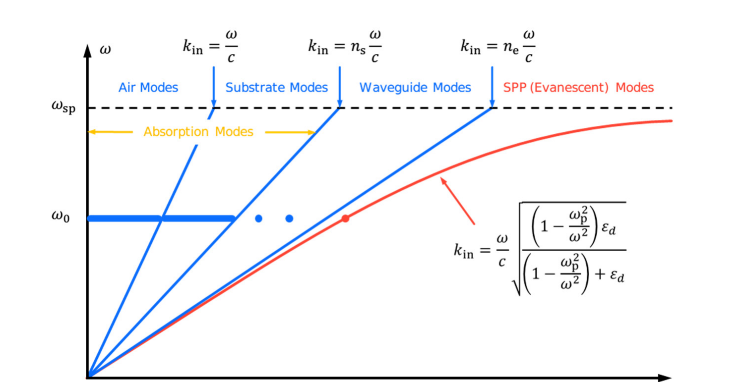
For $u\le1$ , a real propagation angle exists inside the EML. For $u>1$ , the normal wavevector becomes imaginary, describing a field that propagates along the interface and decays exponentially away from it. A uniaxial birefringent EML uses the corresponding ordinary or extraordinary index to normalize each component.

Air, substrate, waveguide, and surface-plasmon regions in frequency and in-plane-wavevector space — Figure 2 | Material light lines define the air, substrate, and EML propagation boundaries; guided and evanescent modes appear at larger in-plane wavevectors.

From Dissipated-Power Spectrum to Mode Fractions

At a fixed wavelength and dipole condition, let the dissipated-power spectrum be $K(k_{\parallel})$ . Narrow peaks usually mark guided-mode or SPP resonances, while the broad background contains propagating waves and material absorption. Integrating over a selected interval gives its raw channel power. Integrating all electromagnetic intervals gives the normalized dissipated power, or Purcell factor:

F=\int_0^\infty K(k_{\parallel})\,\mathrm dk_{\parallel}.

Here, $F$ is normalized to a homogeneous reference environment; the normalization of $K$ includes the corresponding reference power and variable scale. Numerical integration must resolve narrow guided-mode peaks and continue through the evanescent tail until its contribution converges.

The light-line boundaries are

k_t=n_tk_0,\qquad k_b=n_bk_0,\qquad k_s=n_sk_0,\qquad k_e=n_ek_0,

where the subscripts $t$ , $b$ , $s$ , and $e$ denote the top external medium, bottom external medium, finite top-side incoherent substrate, and emissive layer. The largest light line among the propagating channels that actually exist is

k_{\mathrm{esc}}=\max(k_t,k_b,k_s).

An absent bottom-outcoupling or substrate channel is excluded from the maximum.

Mode	Direction and integration interval	Physical meaning
TOC	Top direction, $0\le k_{\parallel}\le k_t$	Light entering the top external medium
BOC	Bottom direction, $0\le k_{\parallel}\le k_b$	Light entering a transparent bottom external medium
SUB	Top direction, $k_t<k_{\parallel}\le k_s$	Light entering the substrate but unable to cross the substrate–external-medium boundary
ABS	Absorptive remainder in the propagating region	Light absorbed by metals or lossy layers before reaching an outcoupling boundary
WVG	$k_{\mathrm{esc}}<k_{\parallel}\le k_e$	Power confined in the films by total internal reflection and transverse resonance
EVA	$k_{\parallel}>k_e$	Evanescent coupling, usually including metal-interface SPP and near-field loss
NRA	No wavevector interval	Nonradiative fraction after emissive excitons have formed

TOC and BOC may occupy the same numerical $k_{\parallel}$ interval because they refer to opposite propagation directions. ABS is also not a separate high-wavevector band; it is the propagating-region power minus power that has crossed an external boundary:

M_{\mathrm{ABS}}=D_{\mathrm{prop}} -M_{\mathrm{TOC}}-M_{\mathrm{SUB}}-M_{\mathrm{BOC}},

where $D_{\mathrm{prop}}$ is the total upward and downward power fraction in the propagating region, and $M_c$ is the normalized fraction of mode $c$ . A channel absent from the structure contributes zero.

Mode Fractions and Device Efficiency

For one emitter, the six electromagnetic channels and the exciton nonradiative channel satisfy

\sum_{c\in\{\mathrm{TOC,BOC,SUB,ABS,WVG,EVA}\}}M_c =q_{\mathrm{eff}}, \qquad M_{\mathrm{NRA}}=1-q_{\mathrm{eff}},

and therefore

\sum_c M_c+M_{\mathrm{NRA}}=1.

Here, $q_{\mathrm{eff}}$ is the effective quantum efficiency and $M_{\mathrm{NRA}}$ is the nonradiative fraction after exciton formation. If the top external medium is air, the conditional top outcoupling efficiency is

\eta_{\mathrm{out,top}}=\frac{M_{\mathrm{TOC}}}{q_{\mathrm{eff}}},

and the top device EQE is

\eta_{\mathrm{EQE,top}}=C\,M_{\mathrm{TOC}} =Cq_{\mathrm{eff}}\eta_{\mathrm{out,top}}.

Here, $C$ is the conversion efficiency from charges to emissive excitons. The loss $1-C$ occurs before exciton formation and is not Mode NRA; NRA covers only material nonradiative decay of excitons that have already formed.

Photon Fractions and Power Fractions

Photon-number and radiant-power spectra are related by the energy of one photon:

\Lambda_P(\lambda)=\Lambda_N(\lambda)\frac{hc}{\lambda}.

Here, $\Lambda_N$ is photon-number weight per unit wavelength, $\Lambda_P$ is radiant-power weight, $h$ is Planck's constant, and $c$ is the speed of light in vacuum. LEE and EQE count photons, so cross-wavelength Mode averages use $\Lambda_N$ . Power Dissipation, Intensity, and color are derived from energy spectra and use $\Lambda_P$ . The same physical emission spectrum should produce the same conclusion whether supplied as photon number or power after the correct conversion.

Conditions for Mode Partitioning

With a finite incoherent substrate on the top propagation side, the mode boundaries require

n_t<n_s<n_e

; without that substrate, they require

n_t<n_e

. A transparent bottom-outcoupling boundary independently requires

n_b<n_e

. The EML must be coherent and transparent. If these index orders fail, the propagating, guided, and evanescent regions cannot be interpreted using the boundaries above.

The standard mode partition allows one finite incoherent substrate on the outcoupling side. A more complex sequence of incoherent external layers may still be used to calculate the final spectrum, but it cannot retain this simplified set of mode intervals. Read Mode together with Power Dissipation: the fractions show how much energy is lost, while the dissipated-power map shows at which wavelengths and wavevectors the loss occurs.

Next Step

Continue with Purcell Effect to see why integrating all electromagnetic channels also changes emitter lifetime and effective quantum efficiency.

Reference

Chance, R. R.; Prock, A.; Silbey, R. Molecular Fluorescence and Energy Transfer near Interfaces. Adv. Chem. Phys. 1978, 37, 1–65.
Wasey, J. A. E.; Barnes, W. L. Efficiency of Spontaneous Emission from Planar Microcavities. J. Mod. Opt. 2000, 47, 725–741.
Nowy, S.; Krummacher, B. C.; Frischeisen, J.; Reinke, N. A.; Brütting, W. Light Extraction and Optical Loss Mechanisms in Organic Light-Emitting Diodes: Influence of the Emitter Quantum Efficiency. J. Appl. Phys. 2008, 104. https://doi.org/10.1063/1.3043800
Meerheim, R.; Furno, M.; Hofmann, S.; Lüssem, B.; Leo, K. Quantification of Energy Loss Mechanisms in Organic Light-Emitting Diodes. Appl. Phys. Lett. 2010, 97, 275.
Chance, R. R.; Prock, A.; Silbey, R. Comments on the Classical Theory of Energy Transfer. J. Chem. Phys. 1975, 62, 2245–2253.

Microcavity Effect

How a microcavity changes emission spectrum, color, angular distribution, Lambertian behavior, and efficiency

Structure Configuration

Structural modeling, layer stacks, and validation