Interpreting Results

Power Dissipation

Read dissipated power versus in-plane wave vector

This guide introduces Power Dissipation, which uses the in-plane wave vector to show how an emitting dipole couples power into outcoupling, waveguide, and evanescent channels. Use it to locate dominant losses and mode peaks.

Reading the chart

Axes

Axis	Meaning
X-axis	In-plane vector, determined by the In-plane Vector Type selected in the Optics page
Y-axis	K (power coupling coefficient / dissipation spectral density)

Three in-plane vector types are available:

Type	Label	Notes
`Effective Index (nEff)`	Effective Index (nEff)	Default; range 0–2.0, step 0.01
`In-plane k`	In-plane k	Normalized in-plane wavevector; range 0–1, step 0.01
`In-plane u`	In-plane u	Equals sin(θ_e); range 0–1, step 0.01

All three parameterizations describe the same physical quantity. The physical meaning and mode-boundary derivations are covered in Emission Theory.

Polarization and Direction

The legend controls are divided into two groups:

Control	Options
Polarization	`TE` / `TM` / `Total`
Direction	`Total` / `Top` / `Btm`

Total (Direction) = Top + Btm combined
TE sums only transverse-electric components; TM sums only transverse-magnetic; Total (Polarization) = TE + TM

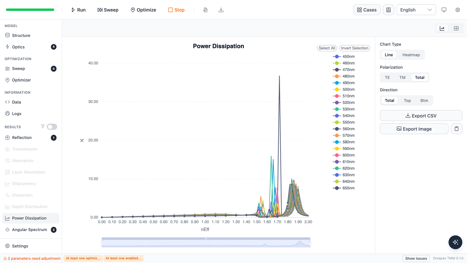
The chart below shows the effect of the Direction control on the power dissipation spectrum:

Direction control example

Spectrum unit and conversion efficiency

The contribution of one emitter to the power-dissipation curve can be written as

D_i(v,\lambda)\propto M_iC_i\Lambda_{P,i}(\lambda)G_i(v,\lambda)

Here, $D_i(v,\lambda)$ is the contribution of emitter $i$ at in-plane coordinate $v$ and wavelength $\lambda$ . $M_i$ is its Multiplication Factor, $C_i$ is its Conversion Efficiency, $\Lambda_{P,i}(\lambda)$ is its radiant-power spectral weight, and $G_i(v,\lambda)$ is the optical response determined by the structure, dipole position, and orientation. Contributions from several emitters are combined in one result; changing emitter order must not change the curve.

When Spectrum Unit is Probability, the photon-number spectrum is converted to a power spectrum:

\Lambda_P(\lambda)=\Lambda_N(\lambda)\frac{hc}{\lambda}

Here, $\Lambda_P(\lambda)$ is the radiant-power spectral density, $\Lambda_N(\lambda)$ is the photon-number spectral density, $h$ is the Planck constant, $c$ is the speed of light in vacuum, and $\lambda$ is wavelength. Spectrum Unit therefore changes the relative strength across wavelength for broad or multi-peak spectra. For one emitter, Conversion Efficiency and Multiplication Factor scale the curve linearly but do not change the mode boundaries at a fixed wavelength.

Spectrum Unit defines the spectral weighting convention; it does not automatically make the vertical axis an absolute W or W/nm quantity. Interpret and export the result using the unit shown on the page.

Wavelength sweep

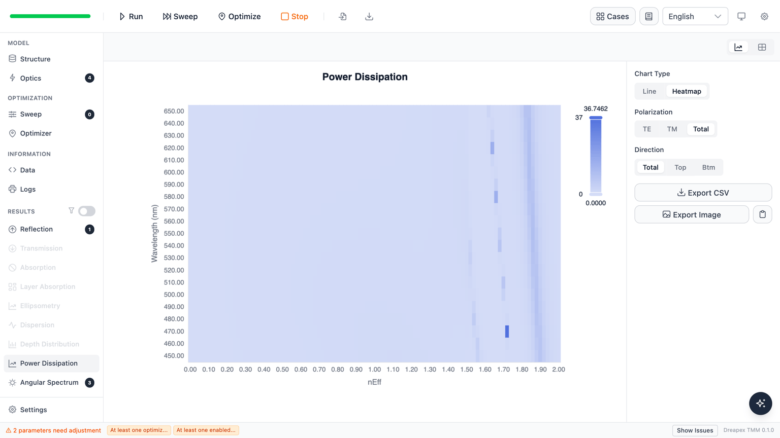
When the Wavelength Mode for the Power Dissipation detector is set to Sweep, the data becomes two-dimensional (in-plane vector × wavelength). Switch to the Heatmap chart type to view the full distribution at once:

Power dissipation heatmap (wavelength sweep)

In the heatmap:

The horizontal axis is the in-plane vector; the vertical axis is wavelength
Color intensity encodes K magnitude
Waveguide modes appear as localized bright bands at characteristic vector values

When the wavelength mode is Single, the chart is fixed to Line; no chart-type toggle is shown.

The Power Dissipation detector does not support the Weighted Average wavelength mode. Only Single and Sweep are available.

Mode boundaries

Several critical values of nEff (or their k/u equivalents) divide the K spectrum into distinct optical mode regions. Using nEff as the axis:

Boundary	Meaning
`nEff = n_s` (substrate index)	Divides substrate modes from waveguide modes
`nEff = n_e` (EML index)	Divides waveguide modes from evanescent (SPP) modes

nEff < n_s: outcoupling region (TOC / BOC)
n_s ≤ nEff < n_e: waveguide modes — light totally internally reflected within the organic stack
nEff ≥ n_e: evanescent modes — predominantly SPP loss

Sharp peaks in the curve correspond to resonant coupling into guided modes; the characteristic peak above nEff = n_e is usually an SPP. The physical derivations and definitions of all mode boundaries are in Emission Theory.

Mode analysis (on the Mode page) requires n_t or n_b < n_s < n_e. If this ordering is not satisfied, the mode-integration boundaries are invalid and Mode page results will be inaccurate.

Controls

Image export and copy (Export Image, Copy Image) and other common controls are shared with every result page — see Basic Optical Results. Page-specific controls:

Control	Description
`Export CSV`	Export all K data (in-plane vector × wavelength × polarization × direction)
Chart type selector	Line or Heatmap — available only in Sweep mode

If the page shows "No data", the most common causes are:

no calculation has been run yet
no layer is marked as emissive (enable the Emis. toggle in the Structure page)
Power Dissipation is not checked in the Emission detector lane of the Optics page

View per-mode energy fractions: Mode
Understand K integration, nEff boundaries, and mode-partition derivations: Emission Theory

Dispersion Results

Phase, group delay, group delay dispersion, and differential group delay

Intensity

Angular and spectral emission intensity, global peaks, envelope FWHM, and normalized views