Limits of the TMM Model
A coating that measures differently from its simulation has not necessarily been calculated wrong. The model itself may not apply to your sample.
TMM rests on a set of idealized premises: interfaces are perfectly smooth, every layer extends without limit sideways, the incident light is a monochromatic plane wave travelling in one direction, and the material response does not depend on intensity. Real samples and real illumination will not satisfy all of them. This chapter lists every premise, the conditions under which each one fails, and the direction in which the simulation then departs from measurement.
Assumptions the TMM Model Relies On
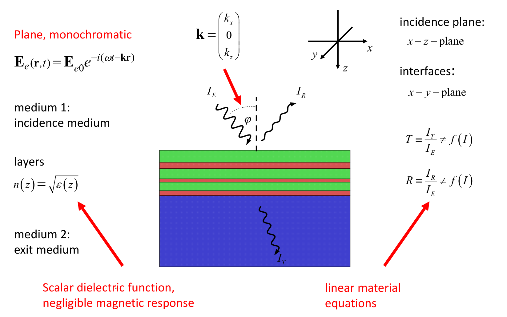
| No. | Assumption | Corresponding input in the software |
|---|---|---|
| 1 | Stratified medium: optical properties vary with depth only, interfaces are ideal planes normal to the depth axis | Layer order and thickness in Structure |
| 2 | Every layer extends to infinity laterally | No input; implied by the model |
| 3 | All media are optically isotropic, magnetic response neglected | Isotropic materials are the default; Birefringent is a controlled relaxation |
| 4 | Incidence and exit sides are semi-infinite homogeneous media, the incidence medium is non-absorbing | Incident and exit media under Surrounding Medium |
| 5 | The incident light is a plane monochromatic wave with a single wavevector | Wavelength and Incident Angle |
| 6 | At oblique incidence the wavevector and the normal define a unique plane of incidence | The s / p definition in Polarization depends on this plane |
| 7 | Three-wave scenario: one incident, one reflected, one transmitted wave | Reflection and Transmission detectors |
| 8 | Materials respond linearly | n and k are independent of intensity |
Nothing in this input list describes light intensity, spot size, beam divergence, or surface roughness — the model has no degrees of freedom for them.
Typical Failure Scenarios
| Real condition | Assumption violated | Observable effect | Direction of the simulation error |
|---|---|---|---|
| Laterally restricted spot (slit, small spot, focused beam) | 5 | The outgoing beam is laterally displaced relative to the incident beam; sub-millimeter shifts have been measured on coatings | Spectral values remain valid, but the beam lands away from where the ideal model implies |
| Focused or defocused conical illumination | 6 | Polarization leakage: p-components mix into nominally s-polarized light | Measured extinction ratio of thin film polarizers falls below the design value |
| Rough interfaces | 1 | Large-scale roughness causes scatter losses; small-scale roughness acts like an antireflection layer | Simulation overestimates specular reflectance and transmittance; no single accepted model exists |
| Layer thickness comparable to the coherence length (thick substrates, broadband sources, limited spectral resolution) | 5 | Interference fringe amplitude is damped; a single spectrum may contain both coherent and incoherent regions | The fully coherent model produces fringes that are too strong |
| Anisotropic materials (glancing-angle deposition, nanolaminates, stretched polymers) | 3 | s and p cannot share one refractive index | An isotropic n fit misses both polarizations at once |
| Spatial dispersion (metal island films, near strong resonances) | Material premise: the response is local | The dielectric function depends on the wavevector | n(λ) is insufficient to describe the material response |
| Time-varying material parameters | Material premise: the response does not change over time | The light frequency is converted; at a temporal interface reflectance plus transmittance can exceed 1 | Outside the range the model can describe |
| High-intensity illumination (pulsed lasers) | 8 | Reflectance and transmittance depend on incident intensity | Linear n, k disagree with high-power measurements |
| Ultrathin films, metal island films, molecular monolayers | Material premise: index and thickness are separable | The spectrum reflects only the product of index and thickness; neither can be fixed on its own | Bulk n, k introduce a systematic bias |
Restricted Spot Size: Displaced Exit Position
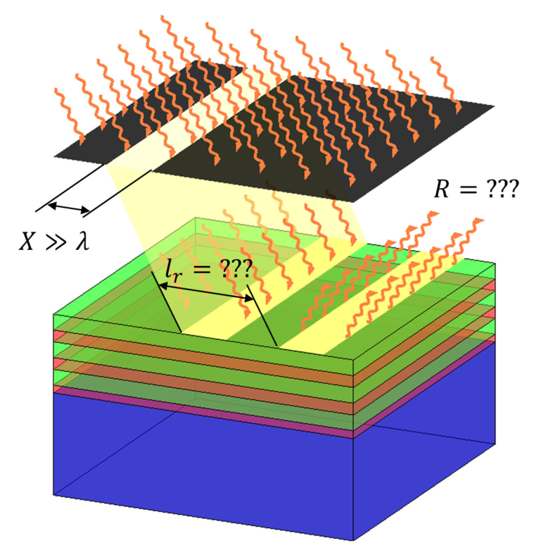
The displacement is set by the derivative of the complex reflection coefficient phase with respect to the incidence angle, so it varies with wavelength and with the coating design. The effect is not confined to total internal reflection: it has been observed near the Brewster angle in p-polarization, at interfaces between transparent and absorbing media, and at metal surfaces. TMM returns reflectance and transmittance values, not the spatial position of the beam; where the spot size and the displacement are comparable, this term has to be budgeted separately.
Conical Illumination: Polarization Leakage
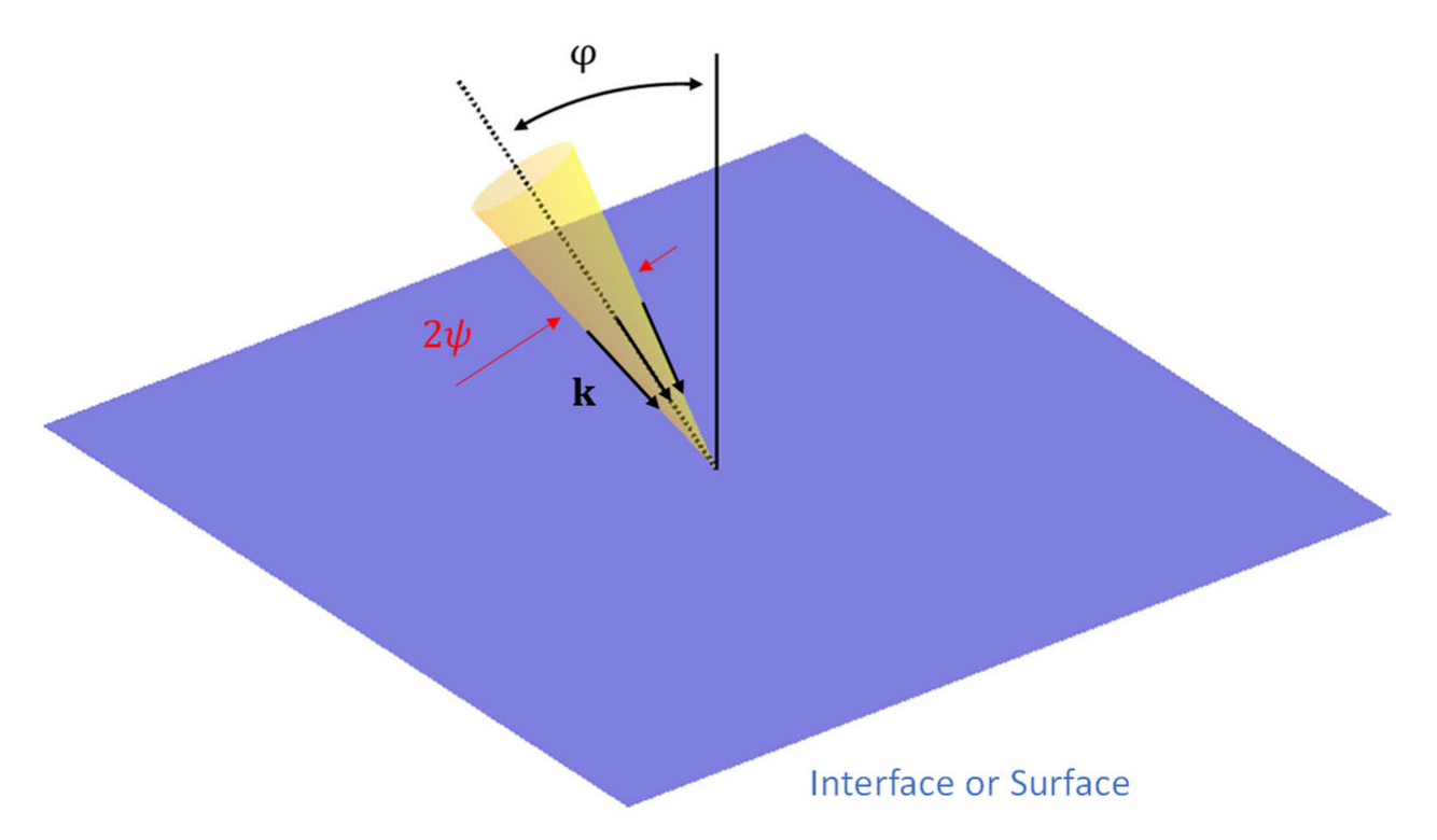
The leakage grows with the cone half-angle and falls as the working incidence angle increases. It is set by the illumination geometry alone, which is why improving the coating design cannot remove it, and why thin film polarizers operating at high incidence angles were developed. When designing polarizing components, treat the simulated extinction ratio as a system upper bound; the achievable value depends on the cone half-angle and the working angle of the illumination system.
Ultrathin Films: Index and Thickness Are No Longer Separable
Whether a layer falls into this regime is set by its single-pass optical phase shift
where is the complex refractive index of the layer, its physical thickness, and the vacuum wavelength; is the phase accumulated in a single pass through the layer.
When , reflectance and transmittance depend only on the product of and . No amount of additional spectra will fix the index and the thickness separately — in a measurement sense they are not two independent quantities. Li and Heinz further note that in this regime the picture of the layer as a uniform slab loses its physical basis: within a film of atomic-scale thickness, the induced currents neither stay uniform through the depth nor switch off abruptly at the boundaries.
Taking as the order of magnitude for entering this regime, the corresponding thicknesses at 550 nm are:
| Material | Thickness |
|---|---|
| Dielectric film with | about 4 nm |
| Metal with | about 2 nm |
The threshold is set by , so there is no universal thickness in nanometers. The same layer can fall on either side depending on the band: a 10 nm gold film reaches above 0.4 in the infrared, which does not satisfy .
The direct consequence for using the software: in this regime an n, k dataset and the thickness assumed when fitting it are a matched pair and have to be used together. Applying optical constants published for one thickness convention to a different thickness introduces a conflict of definition, not a numerical error.
Scenarios Supported by Dreapex TMM
| Capability | Assumption relaxed | Covered | Not covered |
|---|---|---|---|
Cone Angle | 5 (single wavevector) | Weighted average of R / T / A, incident-spectrum-weighted spectra, and color over the cone | Ellipsometry, Depth Distribution, and Dispersion still use a single incidence angle |
Incoherent layers | 5 (fully coherent superposition) | The fully incoherent limit, suitable for thick substrates | The partially coherent regime where thickness and coherence length are comparable |
Birefringent (nExt / kExt) | 3 (isotropy) | Uniaxially anisotropic materials | Mutually exclusive with Incoherent on the same layer |
Surface and interface roughness, scatter losses, spatial dispersion, non-linear response, time-varying materials, thickness-dependent effective optical constants, and lateral beam displacement are not modeled.
Checks Before Running a Simulation
When layer thicknesses are well below the source coherence length, interfaces are smooth, illumination is near-collimated, and intensity stays in the linear range, results can be compared with measured spectra directly. If any of those does not hold, use the three levels below to judge how far the software can help.
Supported, with correct configuration
The software has a matching capability; once it is configured correctly the result holds.
| Check | If this applies | What to do before running |
|---|---|---|
| Coherence length | The stack includes a millimeter-scale substrate, or a broadband source is used | Mark that layer Incoherent; otherwise the spectrum shows dense fringes that do not exist in measurement |
| Material anisotropy | Glancing-angle deposited films, nanolaminates, stretched polymers | Switch to Birefringent and enter nExt / kExt; that layer cannot also be Incoherent |
Supported within a limited range
It can be computed, but only inside a specific range; outside that range the result no longer holds.
| Check | If this applies | What to do before running |
|---|---|---|
| Illumination spread | A focused beam, or collection through a numerical aperture | Enable Cone Angle; it averages intensity only, so a polarizer extinction ratio stays an upper bound |
| Minimum thickness | The single-pass optical phase drops below about 0.1 (at 550 nm, roughly 4 nm for a dielectric, 2 nm for a metal) | Use the n, k that belong with that thickness; the two are a matched pair and cannot be swapped separately |
Not modeled
The software does not cover the physical effect; it requires separate measurement or calculation.
| Check | If this applies | What to do before running |
|---|---|---|
| Surface roughness | The sample has measurable roughness or scatter | Treat the simulated specular reflectance and transmittance as upper bounds and assign the difference to scatter loss |
| Intensity | High-power illumination such as pulsed lasers | Results from linear n, k do not apply to measurements at that power |
Next Steps
Read Transfer Matrix Method for how the model is solved internally, or Optical Parameters to configure cone angle and polarization. For a quantitative comparison against an independent reference under fixed inputs, see Algorithm Validation.
Reference
This chapter follows the published literature below.
Stenzel, O.; Wilbrandt, S. Theoretical Aspects of Thin Film Optical Spectra: Underlying Models, Model Restrictions and Inadequacies, Algorithms, and Challenges. Appl. Sci. 2025, 15, 2187. https://doi.org/10.3390/app15042187 (CC BY 4.0)
Li, Y.; Heinz, T. F. Two-Dimensional Models for the Optical Response of Thin Films. 2D Mater. 2018, 5, 025021. https://doi.org/10.1088/2053-1583/aab0cf