Hole Transport Layers and Thickness Effects in Perovskite Solar Cells

Cuong (2019): ideal photocurrent for two hole transport layers and a perovskite thickness sweep

AuthorLuke Cole

Optical Simulation of Planar CH3NH3PbI3 Perovskite Solar Cells

Author: Nguyen Duc Cuong

Journal: VNU Journal of Science: Mathematics–Physics 35(3), 94–102 (2019) · Comparison targets: ideal photocurrents on p. 101 and the thickness curves in Figure 7c

The hole transport layer of a planar perovskite solar cell lies between the transparent electrode and the perovskite. Its absorption reduces the light reaching the active layer, while layer thickness also changes interference and absorption in the stack. Cuong studied methylammonium lead iodide (MAPbI₃) devices, comparing PEDOT:PSS and copper-doped nickel oxide (Cu:NiOₓ) hole transport layers and calculating how perovskite thickness affects ideal photocurrent.

Page 101 reports the ideal current for a 210 nm absorber in both structures; Figure 7c shows how current varies with thickness. This case uses the material refractive indices provided in Figure 2 to run baseline calculations and 20–500 nm thickness sweeps in Dreapex TMM. Current calculation assumes one electron for each photon absorbed by MAPbI₃, corresponding to 100% internal quantum efficiency.

Commercial figure reuse permission has not been confirmed. See the full paper. Reference currents come from p. 101; thickness-curve data are read from Figure 7c.

Structure

Light enters Glass from air, then passes through the transparent FTO electrode, hole transport layer HEL, MAPbI3, electron transport layer PCBM, and LiF toward the Al back electrode. Both Top Medium and Bottom Medium are air with n of 1. Build the PEDOT:PSS structure first, following the incident-light direction below.

Layer	Thickness	Layer state
Glass	1 mm	`Inco.`
FTO	580 nm	None
HEL	40 nm	None
MAPbI3	210 nm	None
PCBM	50 nm	None
LiF	0.5 nm	None
Al	120 nm	None

FTO is the fluorine-doped tin oxide transparent electrode. PEDOT:PSS is the hole transport material poly(3,4-ethylenedioxythiophene):polystyrene sulfonate; PCBM is a fullerene derivative used for electron transport. HEL uses PEDOT:PSS in the first structure.

Material refractive indices provided in the paper (Figure 2): FTO · PEDOT:PSS · Cu:NiOx · MAPbI3 · PCBM

The paper does not provide refractive indices for LiF or Al. Obtain these data separately for 300–1000 nm.

Each refractive index file contains wavelength in nm, refractive index n, and extinction coefficient k. The five files are extracted from Figure 2 at 5 nm intervals over 300–1000 nm, with reading resolution of approximately 0.006 in n and k.

Open Structure and Add the seven layers. Set Glass to Constant, n of 1.5, k of 0, and enable Inco.. The paper does not specify the glass optical boundary; this case assumes nonabsorbing glass.

For other layers select File, Upload their materials, and use Linear for Interpolation; HEL uses PEDOT:PSS. Disable all Emis. and Tran. switches. Set surrounding media to Constant, named Air-incidence and Air-transmission, with n of 1 and bottom k of 0.

Baseline structure with PEDOT:PSS 40 nm and MAPbI3 210 nm

The screenshot's MAPbI3 and the download mapbi3.nk contain the same data. After upload, the material field displays the filename.

Solar Spectrum

Current integration uses the AM1.5G spectrum from the official Stanford transfer matrix template cited by the paper, retaining its original intensity. AM1.5G denotes the global tilted-plane solar spectrum at air mass 1.5.

Optical Settings

Open Optics and enable Reflectance (R), Transmittance (T), Absorptance (A), and Layer Absorption under Propagation. Both structures use the settings below.

UI field	Setting
`Wavelength Mode`	`Sweep`
`From (nm)`	300
`To (nm)`	1000
`Step (nm)`	1
`Incident Angle`	0°
`Polarization Ratio (p-polarization)`	0.5
`Cone Angle`	Off
`Incident Spectrum`	Off

A polarization ratio of 0.5 gives equal s and p contributions. Material data are linearly interpolated onto the 1 nm calculation grid. With Incident Spectrum disabled, results are absorption fractions; the solar spectrum is used in the subsequent current integration.

Shared 300–1000 nm optical settings for both structures

Optimizer messages about missing optimization objectives and variables do not prevent Run or Sweep in this case.

Baseline Current for Two Hole Transport Layers

Optical current density expresses the current corresponding to sunlight absorbed by the active layer under ideal collection. This case assumes that each photon absorbed by MAPbI₃ produces one collected electron; mA/cm² means milliamperes per square centimeter of device area. The paper uses this convention for its predicted short-circuit current at 100% internal quantum efficiency. Actual short-circuit current also depends on carrier recombination and charge collection.

PEDOT:PSS Structure

Click Run. After completion, open Layer Absorption and select Line. Deselect the other layers in the legend to display only the absorption spectrum of the 210 nm MAPbI3 layer.

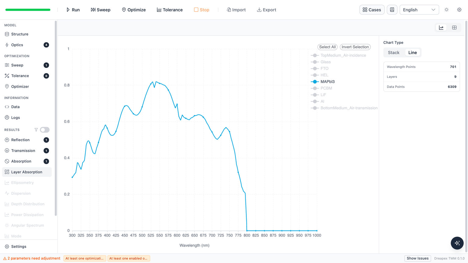
MAPbI3 absorption spectrum in the PEDOT:PSS baseline structure

This figure shows simulation results; the paper provides no corresponding figure.

Dreapex TMM’s Layer Absorption gives the absorption fraction at each wavelength. This case calculates current after exporting the MAPbI3 spectrum: dividing the AM1.5G spectral power by the photon energy at each wavelength gives the incident photon flux; multiplying by MAPbI3 absorption gives the absorbed photon flux. Integration over wavelength and multiplication by the elementary charge give the optical current density used for comparison:

J_{\mathrm{opt}}=0.1q\int_{300}^{1000}A_{\mathrm{act}}(\lambda)S(\lambda)\frac{\lambda_{\mathrm m}}{hc}\,\mathrm d\lambda .

$J_{\mathrm{opt}}$ is optical current density under the ideal collection assumption above, in mA/cm²; $A_{\mathrm{act}}$ is the dimensionless MAPbI3 absorption fraction; $S$ is AM1.5G spectral power density in W/m²/nm. $\lambda$ is wavelength in nm and $\lambda_{\mathrm m}=10^{-9}\lambda$ is wavelength in m.

Multiply the template's solar spectrum values in mW/cm²/nm by 10 to obtain $S$ . The factor 0.1 converts the integrated A/m² to mA/cm².

The elementary charge $q$ , Planck constant $h$ , and vacuum speed of light $c$ are $1.602176634\times10^{-19}$ C, $6.62607015\times10^{-34}$ J·s, and $299792458$ m/s. Linearly interpolate the solar spectrum onto the 1 nm grid and apply trapezoidal integration over 300–1000 nm.

Dreapex TMM simulation data: MAPbI3 absorption spectra for both structures

This structure gives 16.46 mA/cm², compared with 16.59 mA/cm² on paper p. 101, a relative difference of −0.80%.

Cu:NiOx Structure

Return to Structure and change only HEL thickness and material. Retain the baseline values for all other layers, including the 210 nm MAPbI3 thickness.

Change	PEDOT:PSS structure	Cu:NiOx structure
HEL thickness	40 nm	15 nm
HEL material	PEDOT:PSS	Cu:NiOx

Baseline structure with Cu:NiOx 15 nm as HEL

Click Run again and retain only MAPbI3 in Layer Absorption → Line. The same spectrum and integration procedure give 17.86 mA/cm², compared with 17.97 mA/cm² in the paper, a relative difference of −0.64%.

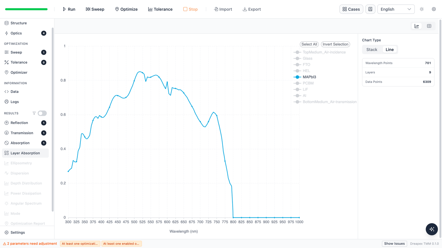
MAPbI3 absorption spectrum in the Cu:NiOx baseline structure

This figure shows simulation results; the paper provides no corresponding figure.

HEL condition, MAPbI3 210 nm	Paper text, mA/cm²	Dreapex TMM, mA/cm²	Relative difference
PEDOT:PSS 40 nm	16.59	16.46	−0.80%
Cu:NiOx 15 nm	17.97	17.86	−0.64%

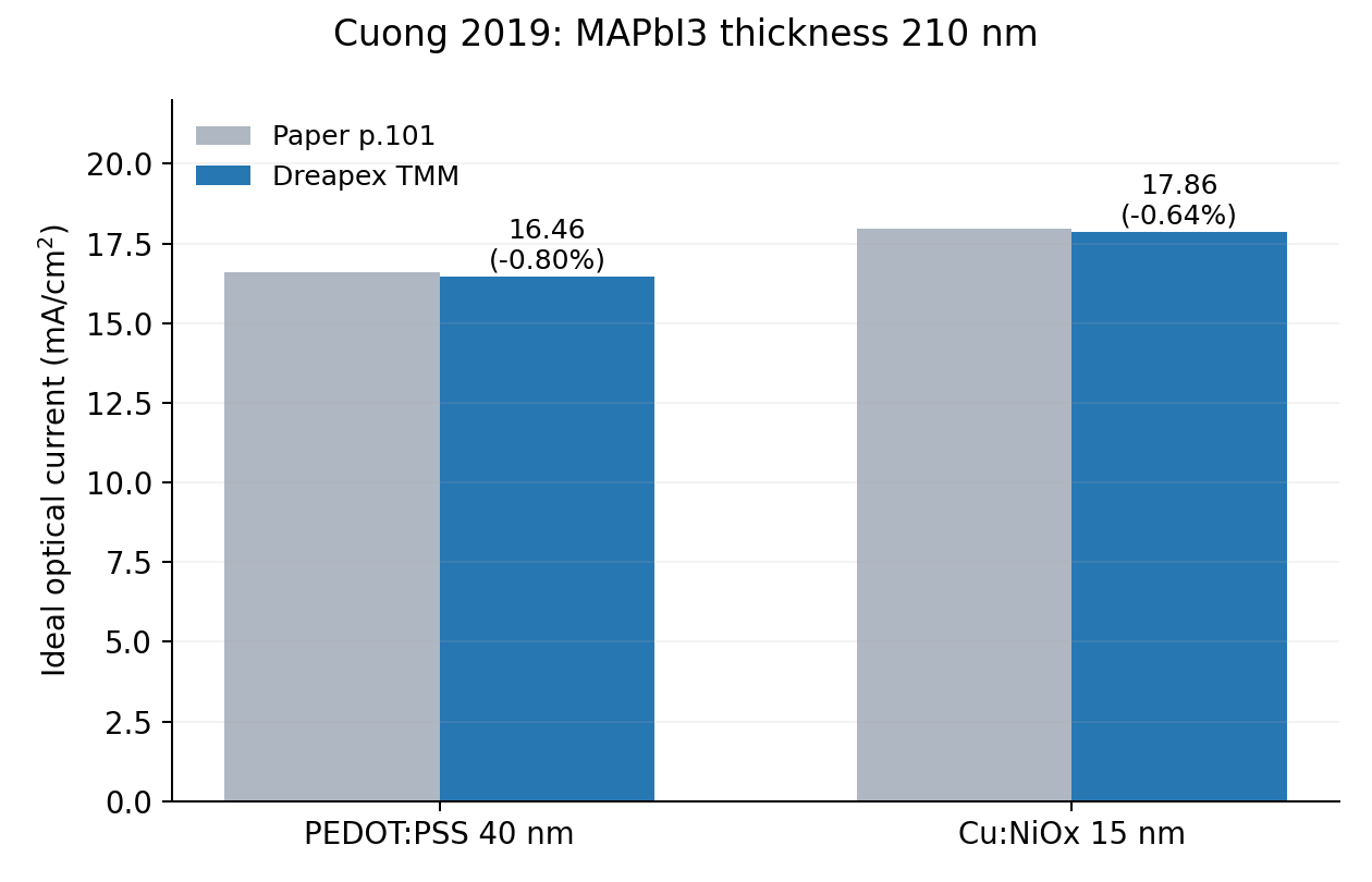
Paper baseline currents and actual integrated spectra for two hole transport layer structures — Gray: values on paper p. 101. Blue: ideal photocurrents from the two baseline calculations above.

Paper text and Dreapex TMM simulation comparison data: two baseline currents

The calculated currents differ by 1.40 mA/cm². With the same integration, HEL parasitic absorption corresponds to 1.97 mA/cm² for PEDOT:PSS and 0.32 mA/cm² for Cu:NiOx. Changing the hole transport layer also changes interface reflection and interference, so the HEL absorption difference is not directly equal to the active-layer current gain.

Perovskite Thickness and Current (Figure 7c)

Thickness Sweep with Cu:NiOx

Retain Cu:NiOx at 15 nm and keep all non-active layers fixed. Open Sweep, use Add to create one sweep item, enable its row, disable Sync, and use the following settings.

UI field	Setting
`Type`	`Single`
`Parameter`	`structure / MAPbI3 / thickness`
`From`	20
`To`	500
`Sampling`	`Step`
`Step`	20

The MAPbI3 thickness unit is nm, giving 25 combinations from 20 to 500 nm at 20 nm intervals.

25-point MAPbI3 thickness sweep settings for the Cu:NiOx structure

Click Sweep in the toolbar. After completion, open Layer Absorption, select Heatmap, and set Layer to MAPbI3. The horizontal axis is wavelength, the vertical axis is absorber thickness, and color indicates active-layer absorption. Click Export CSV to save the spectra for each thickness.

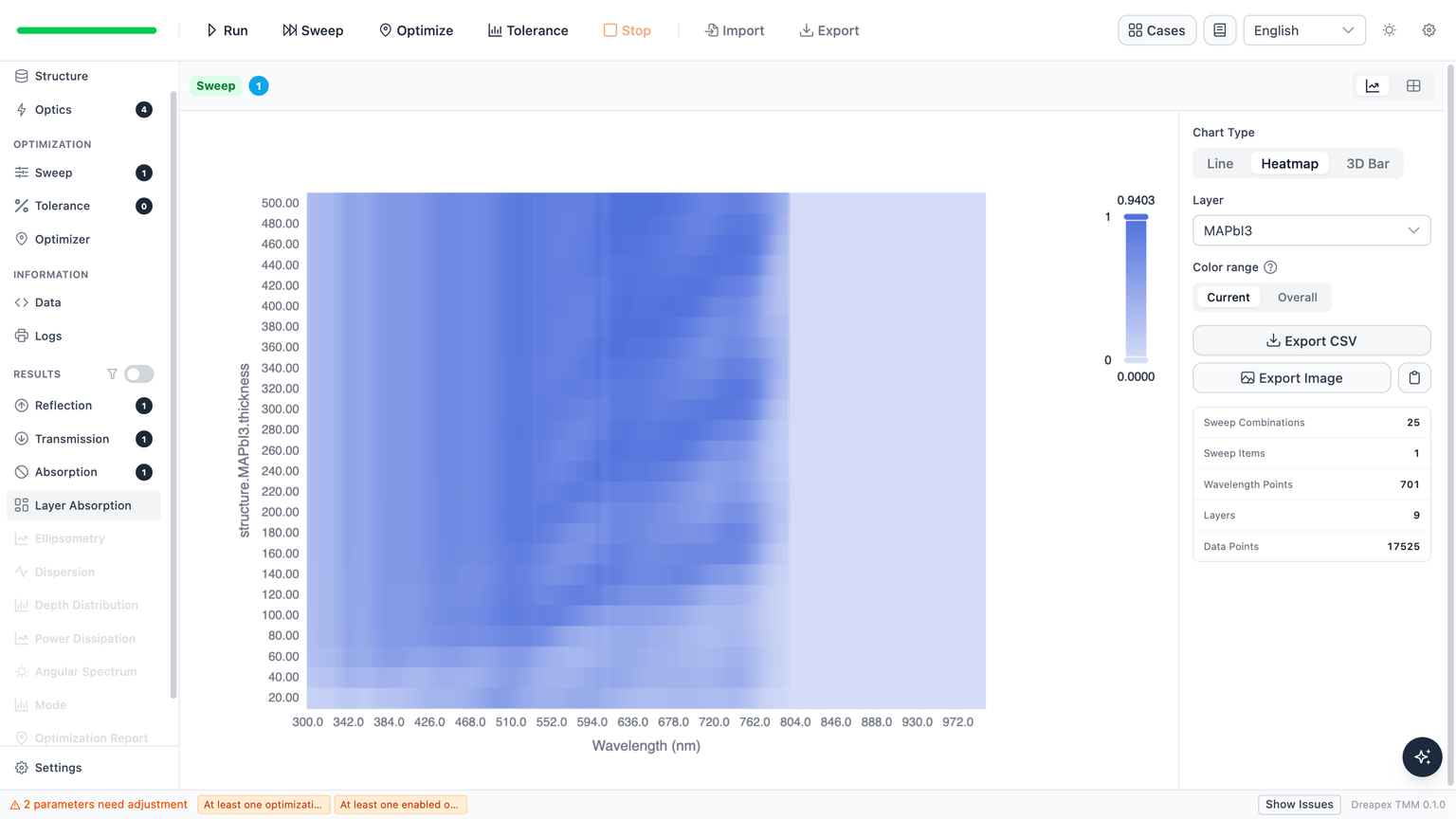
Actual MAPbI3 absorption heatmap versus thickness and wavelength with Cu:NiOx

This figure shows simulation results; the paper provides no corresponding figure.

Thickness Sweep with PEDOT:PSS

Return to Structure and change HEL back to PEDOT:PSS 40 nm. Retain the same MAPbI3 sweep item and all optical settings. Open Sweep, verify the range, and run Sweep again from the toolbar.

Identical MAPbI3 thickness sweep settings for the PEDOT:PSS structure

Select Heatmap and MAPbI3 in Layer Absorption and use Export CSV to save the second set of spectra.

Actual MAPbI3 absorption heatmap versus thickness and wavelength with PEDOT:PSS

This figure shows simulation results; the paper provides no corresponding figure.

Thickness Curve Comparison

Apply the baseline integration equation to each thickness's MAPbI3 spectrum to obtain the solid curves below. Open symbols are data read from Figure 7c, with uncertainty of approximately 0.2 mA/cm². Points obscured by the legend or unresolved curves are excluded from comparison.

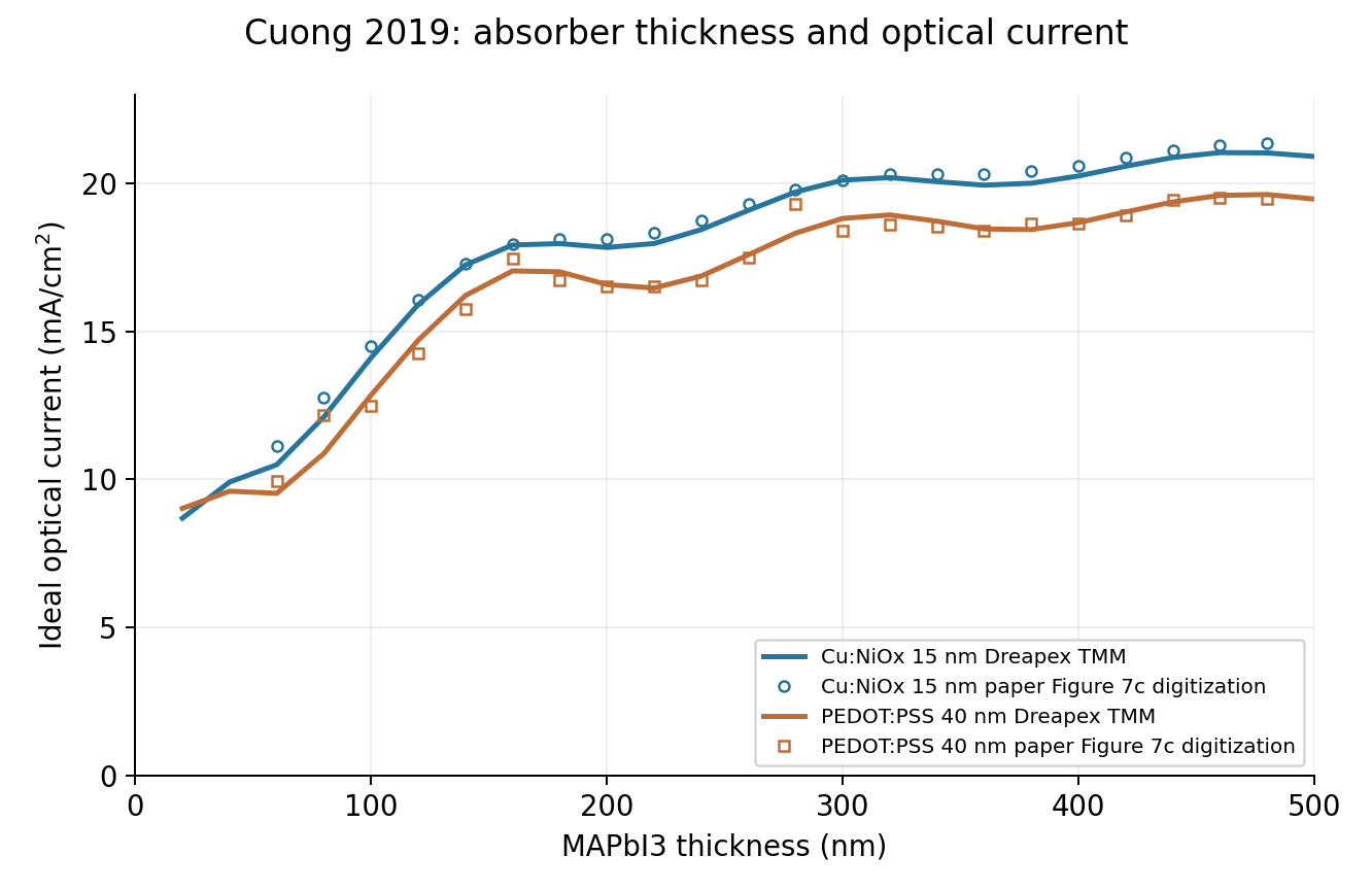
Actual thickness-sweep currents overlaid with digitized Figure 7c values for two hole transport layers — Solid curves: solar-weighted currents from the two actual sweeps. Open symbols: numerical extraction from paper Figure 7c.

Across 20–100 nm, current increases overall with MAPbI3 thickness in both structures; thicker absorbers show interference oscillations. Across the readable paper points included in the statistics from 60 to 480 nm, the Cu:NiOx structure gives higher current than PEDOT:PSS, consistent with the paper. Errors over this range are listed below.

Hole transport layer	Root-mean-square error, mA/cm²	Maximum local difference, mA/cm²
Cu:NiOx	0.32	0.63
PEDOT:PSS	0.43	1.31

Digitized paper and Dreapex TMM simulation comparison data: Cu:NiOx thickness sweep · PEDOT:PSS thickness sweep

Deviation Notes

Five materials' n and k are digitized from Figure 2, with an original 5 nm sampling interval and approximately 0.006 single-pixel resolution. The 1 nm calculation grid is linear interpolation. Baseline currents are 0.80% and 0.64% below the paper values.
The paper does not specify the glass optical boundary. This case uses 1 mm incoherent glass with n of 1.5, k of 0, and air on both sides. Separately sourced LiF and Al data may affect absolute current and the positions of thickness extrema.
Figure 7c reading uncertainty is approximately 0.2 mA/cm²; points below 60 nm are excluded from error statistics. The maximum local sweep difference is 1.31 mA/cm².

Back to Case Studies · Next: One-Dimensional Microcavity Thickness Optimization in a Top-Emitting Micro-OLED